CSPlotter

A Mathematica package for visualizing contact structures in R³.

To use CSPlotter you need to download the file CSPlotter.m and put it in your current working directory in Mathematica. (You may also view the code here.) From the Mathematica prompt, you can then load it by typing

<<CSPlotter.m

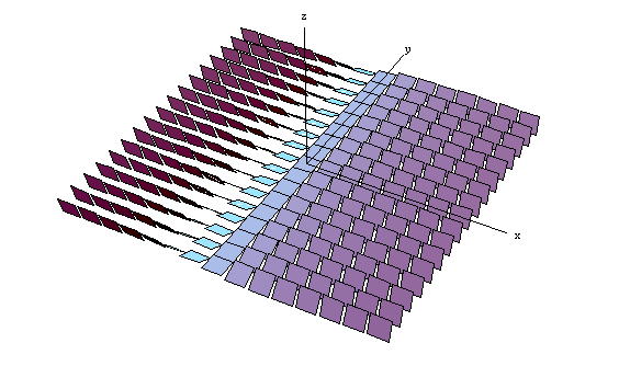
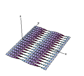
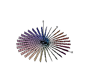
If this generates an error, Mathematica can not find the file CSPLotter.m. The command Directory[] shows what directory Mathematica is currently in, and you can use SetDirectory["/user/mydir"] to change this directory.

Once you have loaded CSPlotter.m, it will provide the command contactelement(pos, v, s) that produces a small tile at pos, normal to v, and of size s. Since at each point in R³ a contact structure is a two dimensional subspace of the tangent space, such tiles can be used to visualize a contact structure in R³ at one point. (The tile shows the orientation of the vector subspace.) By plotting many such tiles, one can visualize the whole contact structure. For example, the standard contact structure ker dz-x dy is visualized using the commands:

xmin = -3.5; xmax = 3.5; dx = (xmax - xmin)/14; ymin = -3.5; ymax = 3.5; dy = (ymax - ymin)/16; size = dy; normal[x_, y_, z_] = {0, -x, -1}; Table[contactelement[{x, y, 0}, normal[x, y, 0], size], {x, xmin, xmax, dx}, {y, ymin, ymax, dy}]; out = Show[%, coords[xmax + 1, ymax + 1, 3.4], Boxed -> False]

This gives the following picture:

Since the contact structure does not depend on z, the structure is only plotted for z=0. In this picture it is clearly seen that at x=0, the tiles are normal to z, and as x becomes non-zero the tiles rotate around the x-axis. The command coords is also provided by CSPlotter. It produces the coordinate axes of variable lengths. For more information on the commands, see the CSPlotter.m source file.

CSPlotter has been tested with Mathematica 5.0.1.0.

More examples

Standard structures [.nb]
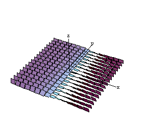
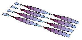
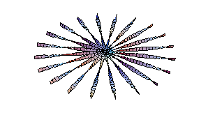
Alternative representation of the standard structures [.nb]
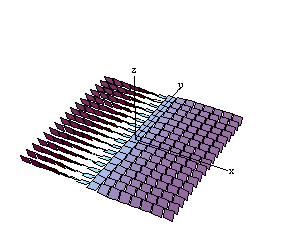
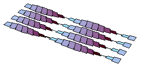
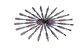
Zoom in of the alternative representation [.nb]
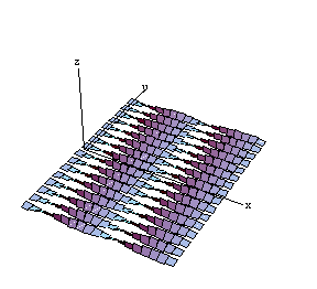
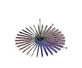
Radial symmetric structures [.nb]
Contact structure tight at infinity [.nb]
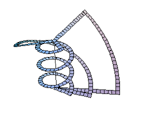
Illustration of Chow's theorem; any two points in the radial symmetric contact structure can be connected [.nb]

Click on the figures for larger figures in .pdf format. All above figures can be found in .eps, .pdf, and .png format in this directory .

Something missing?

All comments, corrections, additions, and improvements are very welcome. For example, if you have plotted another contact structure with CSPlotter, I could put it on this page. My email is matias.dahl at-tkk.fi

Originally, I wrote the routines in CSPlotter to plot contact structures for my Master's thesis, Contact and symplectic geometry in electromagnetics. Variants of some of the above images were used in this paper in PIER.

Keywords: contact structures, visualization of contact structures, pictures of contact structures, mathematica, Chow's theorem, standard contact structure, owertwisted contact structure, tight contact structure, contact structure tight at infinity.