Kanttiaallon approksimointia Fourier-sinisarjan osasummilla
The Fourier series expansion for a square-wave is made up of a sum of odd harmonics, as shown here using MATLAB®.Sisällys
Add an Odd Harmonic and Plot It
t = 0:.1:pi*4;
y = sin(t);
plot(t,y);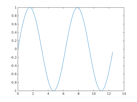
In each iteration of the for loop add an odd harmonic to y. As k increases, the output approximates a square wave with increasing accuracy.
for k = 3:2:9Perform the following mathematical operation at each iteration:
$$ y = y + \frac{\sin kt}{k} $$ aaaaaaaaaaaaaaaaaaaaaaaaaaaaaaaaaaaaaaaaaaaaaaaaaaaaaaaaaaaaaaa
Display every other plot:
    y = y + sin(k*t)/k;
    if mod(k,4)==1
        display(sprintf('When k = %.1f',k));
        display('Then the plot is:');
        cla
        plot(t,y)
    end
When k = 5.0 Then the plot is: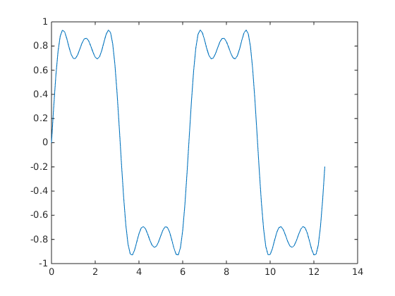 When k = 9.0 Then the plot is:
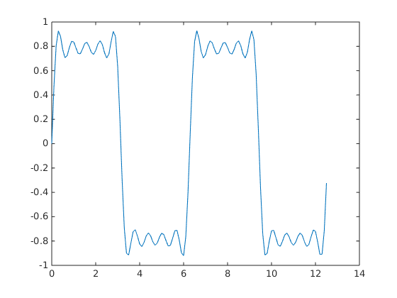
endNote About Gibbs Phenomenon
Even though the approximations are constantly improving, they will never be exact because of the Gibbs phenomenon, or ringing.