Global minimization, 1d, assignment 4 a) Globalminsolve1.m
12.3.2018
apiola@triton:2018kevat/Heikki/Lecture4/
Contents
Function to minimize

Find global minimum (and local minima) on [-2,14]. Split the interval into pieces and use fminbnd on each piece.
Task:
Enlarge interval to [-2,14]
- Change for to parfor, run on pc and Triton, do tic - toc- timing.
- Change to spmd, on Triton you can take more labs than 6.
- Find max-points as well.
Bounds: lb = -2; ub = 14;
Here we will do some more and some less (let's leave the max-part).
clear
close all
format compact
Define objective function:
f = @(x) x.*sin(x) + x.*cos(2.*x)
f =
  function_handle with value:
    @(x)x.*sin(x)+x.*cos(2.*x)
Split into several parts:
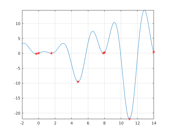
lb=[-2 0 1 3 6 8 10 12];  % Lower bounds
ub=[lb(2:end) 14];  % Upper bounds
% x0=0.5*(lb+ub);     % Starting points for solver that requires them.
N=length(lb);       % Number of subintervals, call them "labs".
%
fminbnd, only bounds are needed.
Basic use: [xmin,ymin]=fminbnd(f,lb,ub);
xmin=zeros(N,1); ymin=xmin; % Preallocation
% parpool;    % Remove comment if pool not open.
tic
% Move commments to parfor and back
% Comment away plot-commands with parfor and when comparing timings.
%for k=1:10   % Take 10 runs to have average timing.
 for i=1:N
 %parfor i=1:N
    [xmin(i),ymin(i)] = fminbnd(f,lb(i),ub(i));
   % %{
     subplot(ceil(N/2),2,i)
    fplot(f,[lb(i) ub(i)]);
     grid on
    hold on
    plot(xmin(i),ymin(i),'ro') % Plot "labwise" minimum point (red circle)
    hold off
   % %}
  end
toc
Elapsed time is 0.432004 seconds.
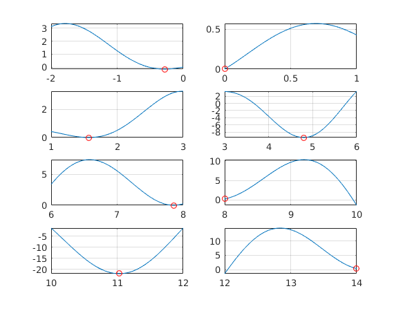
Notice: "Labs" 6 and 8 have the endpointminima wrong, but for the whole the bdary points are often artificial.
%{
N =
    24
Elapsed time is 1.479764 seconds.
Elapsed time is 0.154422 seconds.
%}
minpts=[xmin ymin]
%
minpts =
   -0.2809   -0.1599
    0.0001    0.0001
    1.5708    0.0000
    4.7954   -9.5084
    7.8540    0.0000
    8.0000    0.2538
   11.0318  -22.0274
   14.0000    0.3923
Observations:
- 2^nd (or 3^rd) run is much faster then the 1^st, not to speak about the pool opening run.
- There is little difference with N=8 to N=24 (parfor shows its strength)
- There is little (if any) difference to for, too much overhead compared to intensive computation. Need examples of "heavier" funs and/or bigger data.
%{
 Tfor(k)=toc;
 Tparfor(k)=toc;
 end
 meanTfor=mean(Tfor)
 meanTfor = 0.2513
 meanTparfor=mean(Tparfor)  % First call very slow, setup of pool with workers
 meanTparfor = 0.5459       % Still 2 x slower, gosh!
%}
figure
fplot(f,[lb(1),ub(end)])
hold on
plot(xmin,ymin,'*r');grid on;shg
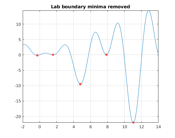
Remove boundarypoints
Here (and often in general) at least some of the boundarypoints are artficial, for the original minimzation problem. Let's remove them.
minpts([2 6 8],:)=[]
figure
fplot(f,[lb(1),ub(end)])
hold on
title('Lab boundary minima removed')
plot(minpts(:,1),minpts(:,2),'r*');grid on;shg
minpts =
   -0.2809   -0.1599
    1.5708    0.0000
    4.7954   -9.5084
    7.8540    0.0000
   11.0318  -22.0274