Contents
Various views of meshgrid
Feb,2018
meshgrid is especially useful for 3d-graphics. Also in any computation where function defined on a 2d-mesh is required.
An easy illustration is to look at a multiplication table.
format compact
close all
Using meshgrid
x=0:2
y=3:6
[X,Y]=meshgrid(x,y);
[X Y]    % X and Y side by side
Z=X.*Y   % Multiplication table
x =
     0     1     2
y =
     3     4     5     6
ans =
     0     1     2     3     3     3
     0     1     2     4     4     4
     0     1     2     5     5     5
     0     1     2     6     6     6
Z =
     0     3     6
     0     4     8
     0     5    10
     0     6    12
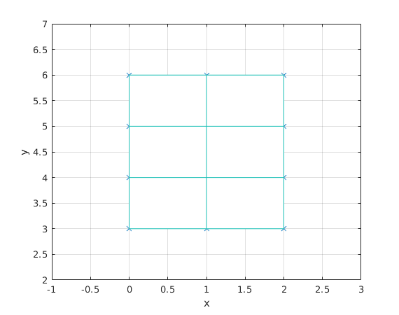
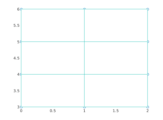
Grid of points
figure
[X(:) Y(:)]
plot(X(:),Y(:),'x')
xlabel('x');ylabel('y')
axis([-1 3 2 7])
hold on
mesh(x,y,0*Z)  % instead of 0*Z, can take 0*X or 0*Y
grid on
ans =
     0     3
     0     4
     0     5
     0     6
     1     3
     1     4
     1     5
     1     6
     2     3
     2     4
     2     5
     2     6
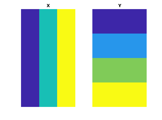
A graphic illustration
figure
subplot(1,2,1)
imagesc(X)
title('X')
axis  off
subplot(1,2,2)
imagesc(Y)
title('Y')
axis off
shg
%
The mesh-command gave an easy way to plot gridlines: mesh(x,y,0*Z) having 2-d-axes open as above.
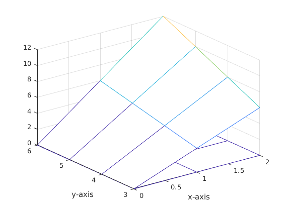
Look at 3d-pictures
That's where you see most uses of meshgrid
figure
mesh(x,y,Z)
xlabel('x-axis')
ylabel('y-axis')
hold on
mesh(x,y,0*Z)
Handy ways to plot gridlines and gridpoints
The easiest way is from above: mesh(x,y,0*Z) % having 2-d-axes open as above
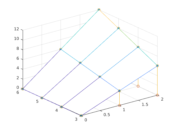
Add grid points and projection lines on the surface
plot3, stem3
figure
plot3(X(:),Y(:),Z(:),'*')
hold on
plot3(X(:),Y(:),0*Z(:),'o')
mesh(x,y,Z)
grid on
stem3(x,y,Z)
shg
% Rotate with your mouse.
Another idea is for 2d-gridlines is to use just ordinary plot
Including some repetition from above. Look at X and Y side by side again:
figure  % New graphics window
plot(X,Y,'k')  % Matlab operates rowwise.
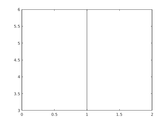
If plot(X,Y) has matrix argumens X,Y of the same size it plots rowwise: plot(X(i,:),Y(i,:)), i=1..m or columnwise plot(X(:,j),Y(:,j)), j=1..n This is a less documented feature. In this case Matlab seems to choose the way that is reasonable looking at the data (sounds a bit incredible). Anyway, it works here, a little confusing, though. Anyway, this procedure is very handy, when you know it.
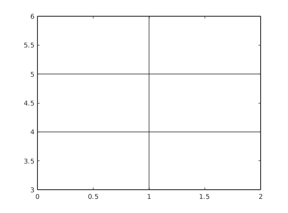
hold on
[X' Y']
ans =
     0     0     0     0     3     4     5     6
     1     1     1     1     3     4     5     6
     2     2     2     2     3     4     5     6
plot(X',Y','k') % Matlab operates columnwise
% (Matlab is 'wise')
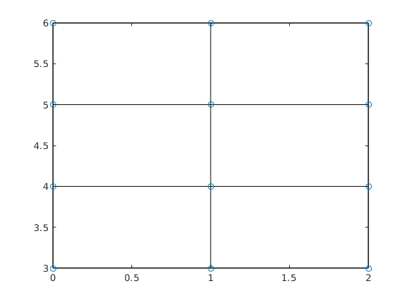
Look at X and Y as long column vectors side by side
[X(:) Y(:)]
ans =
     0     3
     0     4
     0     5
     0     6
     1     3
     1     4
     1     5
     1     6
     2     3
     2     4
     2     5
     2     6
plot(X(:),Y(:),'o')
The gridlines can also be seen most easily in 3d by
mesh(x,y,0*Z)
% You can look directly from above just rotating the figure
% with your mouse.
%
Example of surface plot
Above we considered the function f(x,y)=x y. Instead we could have any function of 2 variables f(x,y) Let's take for instance
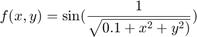
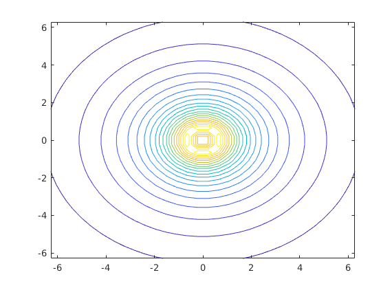
figure
x=linspace(-2*pi,2*pi,30);
y=x;
[X,Y]=meshgrid(x,y);
Z=sin(1./sqrt(.1+X.^2+Y.^2));
mesh(x,y,Z)
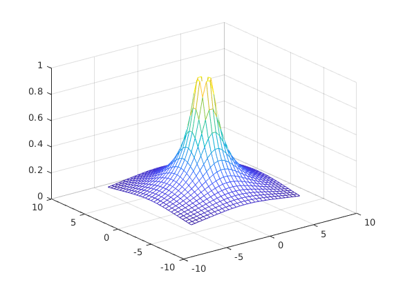
figure
surfc(x,y,Z),colorbar
xlabel('x-axis')
ylabel('y-axis')
contour(x,y,Z,20)
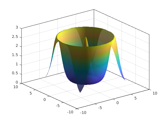
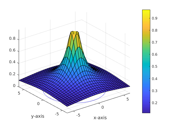
A fancy 3d-plot
Reference:
http://ubcmatlabguide.github.io/html/plottingAdvanced.html
f = @(x,y) exp(cos(sqrt(x.^2 + y.^2))); % Define a function of two variables
d = -2*pi:0.1:2*pi;                     % domain for both x,y
[X,Y] = meshgrid(d,d);                  % create a grid of points
Z = f(X,Y);                             % evaluate f at every point on grid
surf(X,Y,Z);
shading interp;                         % interpolate between the points
material dull;                          % alter the reflectance
camlight(90,0);                         % add some light - see doc camlight
alpha(0.8);                             % make slightly transparent
box on;                                 % same as set(gca,'box','on')