Worksheet 1: The Basics

This homework is designed to teach you to think in terms of matrices and vectors because this is how Matlab organizes data. You will find that complicated operations can often be done with one or two lines of code if you use appropriate functions and have the data stored in an appropriate structure. The other purpose of this homework is to make you comfortable with using help to learn about new functions.

Problem 1.
Problem 2.
Problem 3.
Problem 4.
Problem 5.
Problem 6.
Check solution:
Problem 7.
a
b
c
d
Problem 9.

Problem 1.

Make the following variables

a.) a = 10

b.) b = $2.5 \cdot 10^{23}$

c.) c = 2 + 3i , where i is the imaginary number

d.) d = $e^{\frac{2}{3}\pi\cdot i }$

(Use exp,i,pi)

a = 10
b = 2.5*10^23
% or
b = 2.5e23
c = 2+3i
d = exp(2/3*pi*1i)

a =
    10
b =
   2.5000e+23
b =
   2.5000e+23
c =
   2.0000 + 3.0000i
d =
  -0.5000 + 0.8660i

Problem 2.

a) aVec = [ 3.14 15 9 26 ]

b) bVec = column([2.71 8 28 182]) % column is not a Matlab function.

c) cVec= [ 5 4.8 ... −4.8 −5 ] % (all the numbers from 5 to -5 with increments
of -0.2)

d) dVec = [10^0 10^0.01 ... 10^0.99 10^1]  logarithmically spaced numbers
between 1 and 10.

e) eVec = 'Hello there' (eVec is a string, which is a vector of characters)

aVec = [3.14 15 9 26]
bVec = [2.71; 8 ; 28; 182]
cVec = 5:-0.2:-5;
dVecerr = 10.^0:0.01:1; % Same as 1:.01:1 which gives 1.
dVecerr
dVec=10.^(0:0.01:1);   % We see that power has higher prority than (:)
dVec(1:8)          % 8 first componets of dVec
eVec = 'Hello there'
% Notice the semicolon supressing the large outputs

aVec =
    3.1400   15.0000    9.0000   26.0000
bVec =
    2.7100
    8.0000
   28.0000
  182.0000
dVecerr =
     1
ans =
  Columns 1 through 7
    1.0000    1.0233    1.0471    1.0715    1.0965    1.1220    1.1482
  Column 8
    1.1749
eVec =
Hello there

Problem 3.

Make the following variables:

a)A = 9x9-matrix filled with values 2. Use ones or zeros

b) B= 9x9-matrix with zeros except [1 2 3 4 5 4 3 2 1] on the main diagonal. Use diag (or zeros and linear indexing of type 1:k:81)

c) a 10x10-matrix, where the vector 1:100 runs down the columns. Use reshape

$C = \left [ \begin{array}{cccc} 1&11&\ldots&91\\ 2&12&\ldots&92\\ \vdots&\vdots&\ddots &\vdots\\ 10&20&\ldots&100 \end{array} \right ]$

d) $D = \left[ \begin{array}{cccc} NaN&NaN&NaN&NaN\\ NaN&NaN&NaN&NaN\\ NaN&NaN&NaN&NaN \end{array} \right ]$

e) E=[13 -1 5;-22 10 -87]

f) F = a 5x3-matrix of random integers with values on the range [-3,3]. (use rand, ceil, floor)

A = 2*ones(9)
B = diag([1:5 4:-1:1])
D1 = NaN*ones(3,4);
%or
D2 = NaN(3,4)
% Or:
D3=zeros(3,4)./zeros(3,4);
E = [13 -1 5 ; -22 10 87]
F = fix(8*rand(3,4)-4)
% study the help of fix to figure out what happens

A =
     2     2     2     2     2     2     2     2     2
     2     2     2     2     2     2     2     2     2
     2     2     2     2     2     2     2     2     2
     2     2     2     2     2     2     2     2     2
     2     2     2     2     2     2     2     2     2
     2     2     2     2     2     2     2     2     2
     2     2     2     2     2     2     2     2     2
     2     2     2     2     2     2     2     2     2
     2     2     2     2     2     2     2     2     2
B =
     1     0     0     0     0     0     0     0     0
     0     2     0     0     0     0     0     0     0
     0     0     3     0     0     0     0     0     0
     0     0     0     4     0     0     0     0     0
     0     0     0     0     5     0     0     0     0
     0     0     0     0     0     4     0     0     0
     0     0     0     0     0     0     3     0     0
     0     0     0     0     0     0     0     2     0
     0     0     0     0     0     0     0     0     1
D2 =
   NaN   NaN   NaN   NaN
   NaN   NaN   NaN   NaN
   NaN   NaN   NaN   NaN
E =
    13    -1     5
   -22    10    87
F =
     0    -2    -1    -3
    -1     1     1     3
     1    -2     2     2

Problem 4.

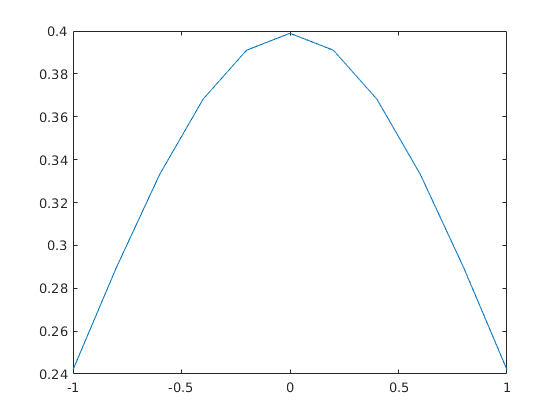
a) Given vector x, evaluate vector y defined by the formula.

$y=\frac{1}{\sqrt{2\pi}}e^{-x^2/2}$

Let x be the interval [-1,1] divided into 10 pieces of equal length and make a plot of y vs. x

Hint: remember to use elementwise operations where needed, i.e. .* and ./ etc.

x = linspace(-1,1,11);
y = 1/sqrt(2*pi)*exp(-x.^2./2);
plot(x,y);shg

Problem 5.

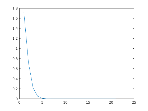
The Taylor expansion of $e^x$ is:

$\sum_{k=0}^{\infty}\frac{x^k}{k!}$

Observe the convergence of the sum with the help of cumsum and exp

x = 1;
k = 0:20;
S = cumsum(x.^k./factorial(k));
plot(abs(S-exp(x)));shg

Problem 6.

Solve the system of linear equations

$\begin{cases}2x+y = 3 \\x-2y = -1\end{cases}$

by using pen and paper; then try out the power of backslash:

A = [2 1; 1 -1]; b = [3;-1];
x = A\b

x =
    0.6667
    1.6667

Check solution:

[A*x b]

%{
ans =
    3.0000    3.0000
   -1.0000   -1.0000
%}

r=A*x - b

%{
r =
   1.0e-15 *    Live editor leaves * out hence hard to interpret result
   0
   0.2220
So "residual" is 10^(-15)*[0;0.222]
%}

ans =
    3.0000    3.0000
   -1.0000   -1.0000
r =
   1.0e-15 *
         0
    0.2220

Using the same technique, solve the system

$\begin{cases} 35 x_1 +14x_3 + 16x_4+ 2x_5 = 67\\ 27x_1 + 7 x_2 + 14x_3 + 4x_4 -7x_5 = 45 \\ -13 x_1 -2 x_2 + 6 x_3 + 10 x_4+ 8x_5 = 9 \\ 30 x_1 -1 x_2 -12 x_3 + 7 x_4 -11x_5 = 13 \\ 7 x_1 + 14 x_2+ 7x_3 -3 x_4 -10x_5 = 15\end{cases}$

A = [35 0 14 16 2 ;
    27 7 14 4 -7;
    -13 -2 6 10 8;
    30 -1 -12 7 -11 ;
    7 14 7 -3 -10 ]
b = [67; 45; 9 ; 13 ; 15]
x=A\b;
x'
[A*x b]
%{
ans =
    1.0000    1.0000    1.0000    1.0000    1.0000
ans =
   67.0000   67.0000
   45.0000   45.0000
    9.0000    9.0000
   13.0000   13.0000
   15.0000   15.0000
%}

A =
    35     0    14    16     2
    27     7    14     4    -7
   -13    -2     6    10     8
    30    -1   -12     7   -11
     7    14     7    -3   -10
b =
    67
    45
     9
    13
    15
ans =
    1.0000    1.0000    1.0000    1.0000    1.0000
ans =
   67.0000   67.0000
   45.0000   45.0000
    9.0000    9.0000
   13.0000   13.0000
   15.0000   15.0000

Problem 7.

Using Matlab indexing, compute the perimeter sum of the matrix "magic(8)".

Perimeter sum adds together the elements that are in the first and last rows and columns of the matrix. Try to make your code independent of the matrix dimensions using "end".

M = magic(8)
S = sum(M(:,1)) + sum(M(:,end)) + sum(M(1,:)) + sum(M(end,:))...
    - A(1,1) - A(1,end) - A(end,end) - A(end,1)

M =
    64     2     3    61    60     6     7    57
     9    55    54    12    13    51    50    16
    17    47    46    20    21    43    42    24
    40    26    27    37    36    30    31    33
    32    34    35    29    28    38    39    25
    41    23    22    44    45    19    18    48
    49    15    14    52    53    11    10    56
     8    58    59     5     4    62    63     1
S =
        1006

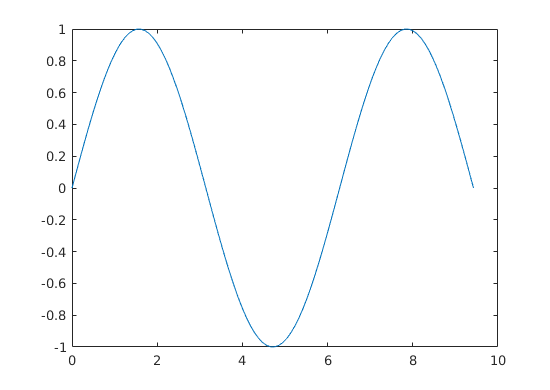
a) Plot the graph of f(x) = sin(x) on interval $[0,3\pi]$

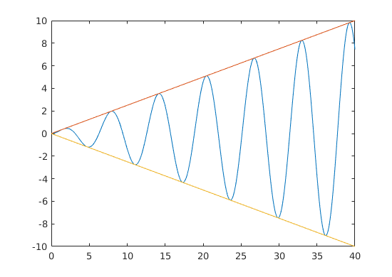
b) Plot the graph of the function $f(x)=\frac{1}{4}x \sin(x) $ on interval [0,40] and in the same picture, plot lines $g_1(x) = \frac{1}{4}x $ and $g_2(x) = -\frac{1}{4}x$ .

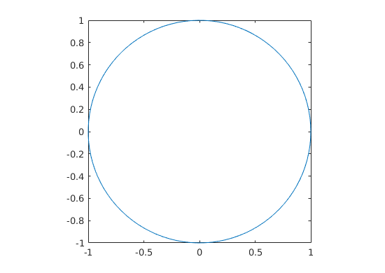
c) Plot a curve with y coordinate of $\sin(t)$ and x coordinate of $\cos(t)$ when $t \in [0,2 \pi]$ .

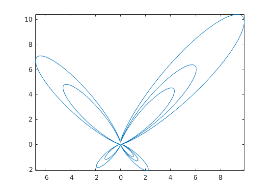
d) Plot a curve

$\begin{cases}x = \sin(t) \left( e^{\cos(t)}- 2\cos(4t) - \sin\left(\frac{t}{12}\right) \right) \\y = \cos(t) \left( e^{\cos(t)}- 2\cos(4t) - \sin\left(\frac{t}{12}\right) \right)\end{cases}$

Test different intervals for t; you'll probably need a fairly long interval.

a

close all
t = linspace(0,3*pi);
plot(t,sin(t))
shg

b

t = linspace(0,40,512);
plot(t,0.25*t.*sin(t),t,t/4,t,-t/4)
shg

c

t = linspace(0,2*pi);
plot(cos(t),sin(t))
axis square
shg

d

t = linspace(0,5*pi,1024);
x = sin(t).*(exp(cos(t) - 2*cos(4*t) - sin(t./12)));
y = cos(t).*(exp(cos(t) - 2*cos(4*t) - sin(t./12)));
plot(x,y)
axis equal
shg
% You may or may not wish to command axis equal for the last two figures,
% depending on your screen.

Problem 9.

Suppose we have

$f(x) = x - e^{-x^2}$

and

$f'(x) = 1+2xe^{-x^2}$

Use Newton's method (teachers and Google will help if you've forgotten what it is) and for or while loop to find the root of $f(x)$ .

f = @(x) x - exp(-x.^2);
df = @(x) 1+2*x.*exp(-x.^2);
x = 1.8;
k = 0;
while(abs(f(x))>0.001)
    k = k +1;
   x = x - f(x)./df(x);
end
k
x
%{
k =
     3
x =
    0.6530
%}