Temperature distribution problem (basic course way)

This is an example of a problem suitable for students in a basic course. It gives one possible line of application for solving systems of linear equations, that can be extended later in many ways (some extensions are more suitable in special courses on numerical PDEs).

Matlab solution

Use pencil and paper to see the structure of the matrix (or just assemble the matrix without seeing any structure).

Assuming you saw something:


>> K=4*diag(ones(4,1))-diag(ones(1,3),1)-diag(ones(1,3),-1)

K =

     4    -1     0     0
    -1     4    -1     0
     0    -1     4    -1
     0     0    -1     4

A1=[K,-eye(4,4),zeros(4,4),zeros(4,4)] 
A2=[-eye(4,4),K,-eye(4,4),zeros(4,4)] 
A3=[zeros(4,4),-eye(4,4),K,-eye(4,4)] 
A4=[zeros(4,4),zeros(4,4),-eye(4,4),K]
A=[A1;A2;A3;A4];
A(1:8,1:8)
>> A(1:8,1:8)    
ans =
     4    -1     0     0    -1     0     0     0
    -1     4    -1     0     0    -1     0     0
     0    -1     4    -1     0     0    -1     0
     0     0    -1     4     0     0     0    -1
    -1     0     0     0     4    -1     0     0
     0    -1     0     0    -1     4    -1     0
     0     0    -1     0     0    -1     4    -1
     0     0     0    -1     0     0    -1     4

>> b=[130,20 10 80 60 0 0 60 40 0 0 40 20 0 0 20]'

Solve the linear equation

>> tvec=A\b                

tvec =

   52.0212
   33.5727
   28.1318
   36.9939
   44.5121
   34.1379
   31.9606
   39.8439
   31.8894
   26.5061
   25.7288
   30.4212
   16.5394
   14.2682
   14.0273
   16.1121

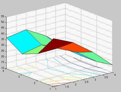
Reshape the solution vector as a 4 x 4 matrix and plot.

tmat=reshape(tvec,4,4)
surfc(tmat); %colorbar  % rotate, see contours etc.







 Continue to Laplace and Poisson equations 


  5- point discretization of Laplacian
 
 General assembly of Poisson equation
 
 Using sparse matrices for large problems (and pcg for solving)
 
 etc.


Solution suggestions