21.4.1999

Assembly prosess step by step in the simplest case

This is an outline of a suggestion for the structure of the solving process. It resembles the structure of the toolbox and (needless to say) uses its data structures. Also the sparse function for building sparse matrices is very handy indeed. Assume our p,e and t are as here, that is run the the Matlab script sess2.m

>> sess2

% export decomposed geometry and boundary cond. from BOUNDARY menu.

[p,e,t]=initmesh(g,'Hmax',5,'jiggle','off');
pdeplotn(p,e,t)

>> t(1:3,:)

ans =

     6     4     1     7     8     9     3     5    10     5     2     7
     1     3     2     5     4     6     6     8     6     9     7    10
    11     9    11    10     9    10     9     9    11    10    11    11

t1ind=t(1:3,1)'
pp1=p(:,t1ind)
hold on
fill(pp1(1,:),pp1(2,:),'g')

Local stiffness matrix

Recall Formula for K_i,j

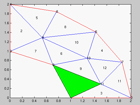
figure
hold on
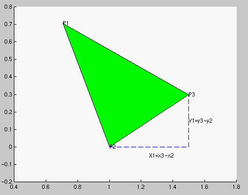
fill(pp1(1,:),pp1(2,:),'g')
axis([0.4 1.8 -0.2 0.8])
text(pp1(1,1),pp1(2,1),'P1')     
text(pp1(1,2),pp1(2,2),'P2')
text(pp1(1,3),pp1(2,3),'P3')
plot(pp1(1,[2,3,3]),pp1(2,[2,2,3]),'--')
text(1.5,0.15,'Y1=y3-y2')
text(1.25,-0.05,'X1=x3-x2')

The above Matlab commands produce this figure where we have the same notation as in PDEtool manual p. 4-6 (With capitalized letters on the LHS). [assem2.gif]


x=pp1(1,:);y=pp1(2,:);
X1=x(2)-x(3);Y1=y(2)-y(3);
X2=x(3)-x(1);Y2=y(3)-y(1);
X3=x(1)-x(2);Y3=y(1)-y(2);

% Here is the "master" (local) matrix Kt, meaning K associated to triangle t.

Kt=[X1*X1+Y1*Y1,X1*X2+Y1*Y2,X1*X3+Y1*Y3;
    X2*X1+Y2*Y1,X2*X2+Y2*Y2,X2*X3+Y2*Y3;
    X3*X1+Y3*Y1,X3*X2+Y3*Y2,X3*X3+Y3*Y3];

[A,a1,a2,a3]=pdetrg(p,t)

Kt=Kt/(4*A(1))

Notice that we get the areas (etc.) of all triangles at once. Let's just check the first one.

det([1,1,1;x;y])/2
A(1)

Remember the area of a triangle formula.

Use the debugger to test your function and to trace the assembly

>> dbstop at 1 in lassema 
>> K=lassema(p,t,f)      
10  nt=size(t,2);      % Nr. of triangles
K>> dbtype
K>> dbstep
K>> dbstep
...

% Look at the local variables, like K .
K> dbclear 1
K> dbquit

Boundary condition matrix b

The boundary condition info is given by the boundary matrix b exported from gui or boundary m-file (like geometry m-file). The former looks in this case like

>> b

b =

     1     1     1     1
     1     1     0     1
     1     1     1     1
     1     1     1     1
     1     1    48     1
     3     3    49     1
    48    48    48    48
    48    48    48    48
    49    49    49    49
    49    49    48    49
    43    43     0     0
   120   121     0     0

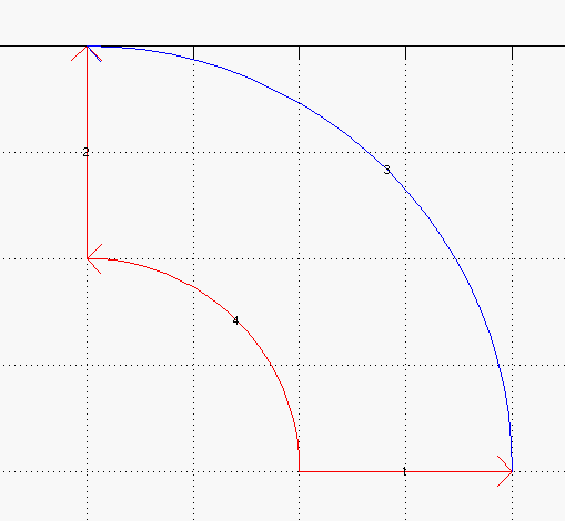
A bit of a mystery, note that 120 is the ascii code for x and 121 for y. What matters for us here is row 2. There 1 means Dirichlet and 0 means Neumann.

>> dirind=find(b(2,:)==1)
dirind =

     1     2     4
>> neuind=find(b(2,:)==0)
neuind =

     3

Choosing "show edge labels" in Boundary menu we see the coincidence. [assembd.gif]

Assembling the stiffness matrix, lassema

Let's follow a similar structure as in the toolbox writing the function lassema (linear as opposed to quadratic that could be called qassema (what would be qubic?) that does the assembly of the stiffness matrix (only that for the time being - we shall restrict ourselves to Poisson at this point).

function K=lassema(p,t)
%
% Assembles the stiffness matrix w.r.t. the mesh defined by p and t.
% p and t can be exported from PDEtool.
%
% This function assembles only the area integral contributions. 
% The function lassemb will take care of the boundaries 
%
% This can be extended into
% function [K,M,F]=lassema(p,t,c,a,f)
% 
% The intermediate step would be a "Poisson assembler"
% 
function [K,F]=lassema(p,t,f)
%
nt=size(t,2);         % Nr. of triangles
np=size(p,2);         % Nr. of points

K=sparse(np,np);     % Initialize stiffness matrix

for n=1:nt   % The big (and only) loop running through each element,
             % i.e. each triangle t.
             
       tri=t(1:3,n);  The local current triangle
       pt=p(:,tri);

%      Form the local matrix Kt (see above)

%      How to find the right slots in the global K where to add the current 
%      contribution?
       
%      Here's a nice trick, be sure to understand it.
       ii=tri(:,[1 1 1])  % One way to repeat the column 3 times
       jj=ii'
       [ii(:) jj(:)]   % This is just for you to see what's going on
       
%      Now comes the main point, the update step of K
       K=K+sparse(ii(:),jj(:),Kt(:),np,np);
       full(K)    % For your display, to be removed
 
end;

%%%%%%%%%% and of assembly of K (version 1 of lassema) %%%%%%%%%%%%%%%%%%%

Now the RHS

Here we can use the mid point rule (accuracy is consistent with linear basis functions (see [E-E-H-J] p. 340). That means simply:

One way to get the barycenters would be as follows. Please give an explanation of what happens here. (I'm sorry to do all this for you but it makes me sick to see unnecessary complicated loop constructructions. Of course you might find another way of reshaping the data.) Also plot the points to see they go right.


% RHS
tri_ind=t(1:3,:);tri_ind=tri_ind(:);
x=p(1,tri_ind)';y=p(2,tri_ind)';
x3=reshape(x,3,nt);y3=reshape(y,3,nt);
x=sum(x3)/3;y=sum(y3)/3;

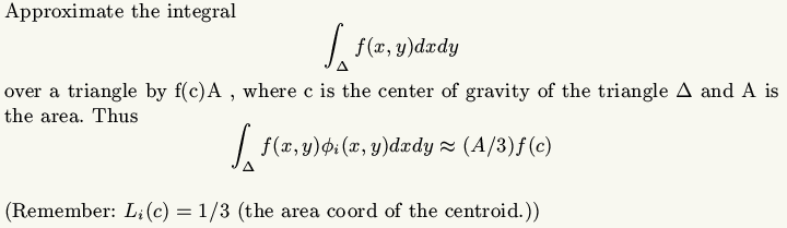
When using the mid-point integration rule we evaluate the function f at the barycenters. Now, remember that the f in the toolbox is given as a string of type f='x.^2+y.^2' or f='0' or f:='ff(x,y)' , where ff is an m-file ff.m. In any case (more precisely in the non-constant case) the symbols x and y are used as argument names for the function. (A bit questionable but convenient)

Hence f=eval(f) gives the vector of values at the barycenters. Here it was necessary to use the names x and y for the vectors of x- and y- coordinates of the barycenters respectively.

(Note that in the general elliptic case the coefficient functions c and a are treated similarly.)

Thus we could continue :

f=eval(f)
F=zeros(np,1);
if any(f)  % Test if there's any non-zero component
  for i=1:nt  % Only this loop is needed, as in the stiffness matrix case.
  ..
  end;
end;

So there is just to fill in the details, add comments and test. You could even write a demo that shows also graphically the process triangle by triangle.

Note that this is totally independent of the geometry.

A more general case

Before going into this it is perhaps a good idea to complete the Poisson solver with the adjustments caused by the boundaries.

Let's take the generalizations for lassema here anyway now.


function K=lassema(p,t,f)      % 1. version  (Poisson)
%function [K,F]=lassema(p,t,f) % 2. version  (Poisson)
%function [K,M,F]=lassema(p,t,c,a,f) % Final version for general elliptic
%
% Assembles the stiffness matrix w.r.t. the mesh defined by p and t.
% p and t can be exported from PDEtool.%
% This function assembles only the area integral contributions. 
% The function lassemb will take care of the boundaries %
%
% The final version returns area integral contributions of 
% 1. stiffness matrix K
% 2. mass matrix M
% 3. RHS F

Continue with boundary assembly