Global minimization, 1d, assignment 4 a)
9.3.2018
Contents
Function to minimize

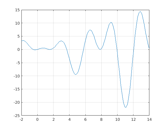
Find global minimum (and local minima) on [0,12]. Split the interval into pieces and use fminbnd on each piece. Bounds: lb = -2; ub = 14;
clear
close all
format compact
Define obj function
f = @(x) x.*sin(x) + x.*cos(2.*x)
f =
  function_handle with value:
    @(x)x.*sin(x)+x.*cos(2.*x)
Split into several parts:
lb=[-2 0 1 3 6 8 10 12];  % Lower bounds
ub=[lb(2:end) 14];  % Upper bounds
x0=0.5*(lb+ub);     % Starting points for solver that requires them.
close all
fminbnd, only bounds are needed, no starting points.
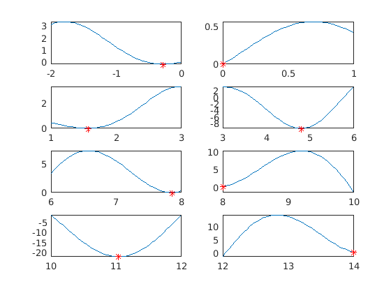
x=zeros(8,1); y=x;
tic
for i=1:8
    [x(i),y(i)] = fminbnd(f,lb(i),ub(i));
    subplot(4,2,i)
    fplot(f,[lb(i) ub(i)]);
    grid on
    hold on
    % plot(x0(i),f(x0(i)),'k+') % For solver that needs init. points.
    plot(x(i),f(x(i)),'ro') % Plot "labwise" minimum point (red circle)
    hold off
    %title(['Bounds: [',num2str(lb(i)),',',num2str(ub(i)),']'])
end
T(1)=toc
minpts=[x y]
T =
    0.5397
minpts =
   -0.2809   -0.1599
    0.0001    0.0001
    1.5708    0.0000
    4.7954   -9.5084
    7.8540    0.0000
    8.0000    0.2538
   11.0318  -22.0274
   14.0000    0.3923
Compare with using just Malab's vector function min.
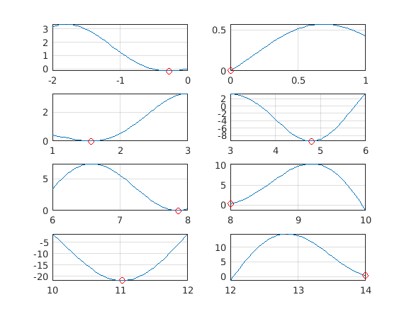
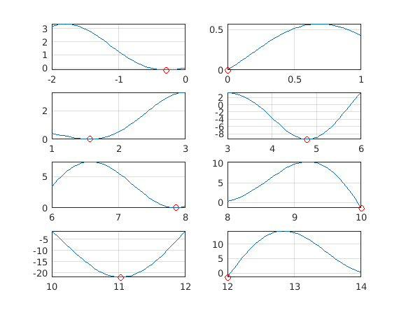
figure
tic
for i=1:8
    xx=linspace(lb(i),ub(i));
    yy=f(xx);
    ymin=min(yy);
    Yes=(yy==ymin);  % Better test: abs(yy-ymin)< tol, see later
    xmins{i}=xx(Yes);
    ymins{i}=yy(Yes);
    subplot(4,2,i)
    fplot(f,[lb(i) ub(i)]);
    grid on
    hold on
    plot(xmins{i},ymins{i},'ro') % Plot "labwise" minimum point (red circle)
    hold off
end
T(2)=toc
xmins
ymins
T =
    0.5397    0.4134
xmins =
  1×8 cell array
  Columns 1 through 7
    [-0.2828]    [0]    [1.5657]    [4.7879]    [7.8586]    [10]    [11.0303]
  Column 8
    [12]
ymins =
  1×8 cell array
  Columns 1 through 6
    [-0.1598]    [0]    [6.2040e-05]    [-9.5077]    [2.4989e-04]    [-1.3594]
  Columns 7 through 8
    [-22.0274]    [-1.3487]
Simple vector operation was about just as fast and all results were correct, in contrary to fmincon. On "labs" 6 and 8 fmincon gets the endpoint values wrong in these cases.
If you wants to increase accuracy, you will do better by adjusting the tolerances with optimset, and running fmincon with tight intervals (obtained with logical indexing as above).
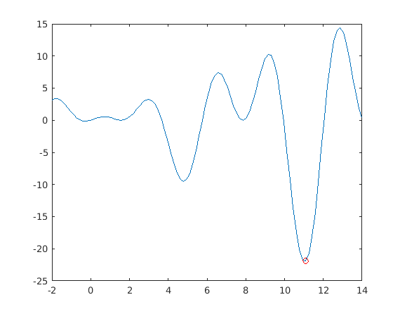
Global minimum using Matlab's [ymin,minind]=min(f(x)).
This is a couple of lines shorter than the above logical indexing way. On the other hand it misses the rest of several (almost) equal minimums. In this case works fine.
figure
u=linspace(lb(1),ub(end));
[ymin,imin]=min(f(u))         % Picks first min-value and its index.
plot(u,f(u),u(imin),ymin,'ro')
ymin =
  -21.9305
imin =
    82
%{
figure
[ymin,imin]=min(f(x))   % Picks first min-value and its index.
xmin=x(imin)
%}
%{
figure
xx=linspace(lb(1),ub(end));
plot(xx,f(xx),x,f(x),'ro')
grid on
%}
Task:
Enlarge interval to [-2,14] (a) Change for to parfor, run on pc and Triton, do tic - toc- timing. (b) Change to spmd, on Triton you can take more labs than 6. (c) Find max-points as well.
pc/Triton (Brute)
To use spmd, we need a form whose argument list is a 2-vector instead of two scalars.
fminbndI=@(f,Interval) fminbnd(f,Interval(1),Interval(2))
fminbndI =
  function_handle with value:
    @(f,Interval)fminbnd(f,Interval(1),Interval(2))
u=linspace(lb(1),ub(end));
%[ymin,imin]=min(f(u))         % Picks first min-value and its index.
% plot(u,f(u),u(imin),ymin,'ro')
plot(u,f(u));grid on
nlabs=2;
nlabs=8;     %  brute: max = 12, triton: max=24
p=parpool(nlabs);
Starting parallel pool (parpool) using the 'local' profile ... connected to 8 workers.
tic
spmd
   % intervals=[-2 3;3 8]
    intervals=[lb' ub'];
    Int=intervals(labindex,:);
    [x,y]=fminbndI(f,Int);
end
Tspmd=toc
% Varies a bit, the first is a lot slower.
%{
Tspmd =
    1.0614
Tspmd =
    0.1692
%}
Tspmd =
    1.1339
hold on
for k=1:nlabs
    plot(x{k},y{k},'*r')
end
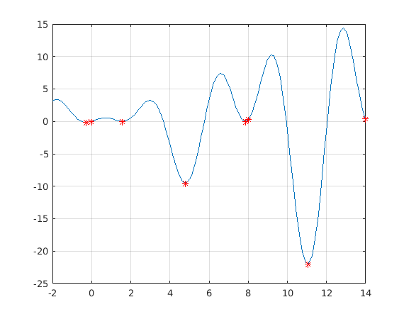
figure
for k=1:nlabs
    subplot(4,2,k)
    fplot(f,[lb(k) ub(k)])
    hold on
    plot(x{k},y{k},'*r')
end