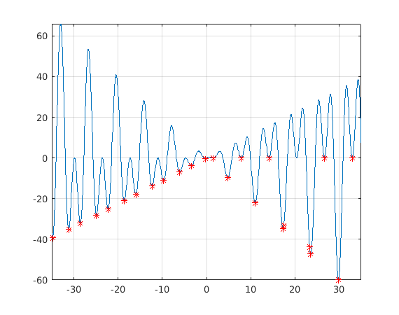
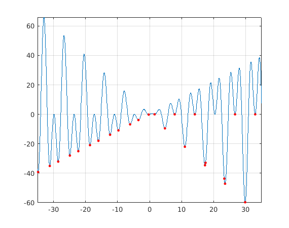
Global minimization, 1d, assignment 4 a), parallel (parfor, spmd)

12.3.2018
apiola@triton:2018kevat/Heikki/Lecture4/Globalminsolve2.m

Continuation to Globalminsolve1.m

Contents

Function to minimize

Find global minimum (and local minima) on [-2,14]. Split the interval into pieces and use fminbnd on each piece.

Task:

Enlarge interval to [-2,14] (a) Change for to parfor, run on pc and Triton, do tic - toc- timing. (b) Change to spmd, on Triton you can take more labs than 6. (c) Find max-points as well. Bounds: lb = -2; ub = 14;

Here we will do some more and some less (let's leave the max-part).

clear
close all
format compact

Define objective function:

f = @(x) x.*sin(x) + x.*cos(2.*x)

f =
  function_handle with value:
    @(x)x.*sin(x)+x.*cos(2.*x)

Split into several parts:

%{
lb=[-2 0 1 3 6 8 10 12];  % Lower bounds
ub=[lb(2:end) 14];  % Upper bounds
% x0=0.5*(lb+ub);     % Starting points for solver that requires them.
N=length(lb);       % Number of subintervals, call them "labs".
%}

Let's make use of all 24 workers on Triton, take wider range.

Remove(d) comments for this 2^nd run

Low=-35;Up=35;N=24;
lb=linspace(Low,Up,N+1);
ub=lb(2:end);
lb=lb(1:end-1);

fminbnd, only bounds are needed, no starting points.

Basic use: [xmin,ymin]=fminbnd(f,lb,ub);

xmin=zeros(N,1); ymin=xmin;
% parpool;    % Remove comment if pool not open.
tic
% Move commments to parfor and back
% Comment away plot-commands with parfor and when comparing timings.
%for k=1:10   % Take 10 runs to have average timing.
 %for i=1:N
 parfor i=1:N
    [xmin(i),ymin(i)] = fminbnd(f,lb(i),ub(i));
    % No graphics now.
    %{
    subplot(ceil(N/2),2,i)
    fplot(f,[lb(i) ub(i)]);
     grid on
    hold on
    plot(xmin(i),ymin(i),'ro') % Plot "labwise" minimum point (red circle)
    hold off
   %}
  end
toc
%{
N =
    24
Elapsed time is 1.479764 seconds.
Elapsed time is 0.154422 seconds.
%}

Elapsed time is 0.866446 seconds.

Observations:

Tfor(k)=toc; Tparfor(k)=toc; end meanTfor=mean(Tfor) meanTfor = 0.2513 meanTparfor=mean(Tparfor) % First call very slow, setup of pool with workers meanTparfor = 0.5459 % Still 2 x slower, gosh!

minptspar=[xmin ymin];

close all

figure
fplot(f,[Low,Up])
hold on
plot(xmin,ymin,'*r');grid on;shg
%

Parallel computing with spmd

spmd

My very first spmd-block

spmd
    Lind=labindex;
end
Lindcell=Lind(1:5)   % First five cells
Lindvect=[Lind{:}]
%
% To use spmd with fminbnd, we need a form whose argument list is a
% 2-vector instead of two scalars. So, here:
fminbndI=@(f,Interval) fminbnd(f,Interval(1),Interval(2))
% (On the 2-variable optimization we need the converse.)
%

Lindcell =
  1×5 cell array
    {[1]}    {[2]}    {[3]}    {[4]}    {[5]}
Lindvect =
  Columns 1 through 13
     1     2     3     4     5     6     7     8     9    10    11    12    13
  Columns 14 through 24
    14    15    16    17    18    19    20    21    22    23    24
fminbndI =
  function_handle with value:
    @(f,Interval)fminbnd(f,Interval(1),Interval(2))

tic
spmd
    intervals=[lb' ub'];
    Int=intervals(labindex,:);
    [xminspmd,yminspmd]=fminbndI(f,Int);
end
Tspmd=toc   % 0.24...   Slightly better than for, twice faster than parfor.
%           % And NOTE the ELEGANCE!
minpts_spmd=[xminspmd{:};yminspmd{:}]; % From workers to client.
%

Tspmd =
    0.4513

figure
fplot(f,[-35,35]);grid on
hold on
plot(minpts_spmd(1,:),minpts_spmd(2,:),'.r','MarkerSize',10)
shg

Compare with using just Matlab's vector function min.

%figure
tic
for i=1:N
% parfor i=1:N
    xx=linspace(lb(i),ub(i));
    yy=f(xx);
    ymin=min(yy);
    Yes=(yy==ymin);  % Better test: abs(yy-ymin)< tol, see later
    xmins{i}=xx(Yes);
    ymins{i}=yy(Yes);
    %{
    subplot(4,2,i)
    fplot(f,[lb(i) ub(i)]);
    grid on
    hold on
    plot(xmins{i},ymins{i},'ro') % Plot "labwise" minimum point (red circle)
    %hold off
    %}
end
display(N)
Tfor=toc      % 0.005
%Tparfor=toc  % 0.14...
minptsvecop=[xmins{:};ymins{:}];

N =
    24
Tfor =
    0.0206

Comments, conclusions, visions

Simple vector operation was about as fast (or even faster) and all results were correct, contrary to fmincon, which got the endpoint values on "labs" 6 and 8 wrong (N=8).

If you want to increase accuracy, you will do better by adjusting the tolerances with optimset, and running fmincon with tight intervals (obtained with logical indexing as above).

Vector operations are so fast that using this technique there's little point in splitting them up into "labs" in case only global minimum is sought unless the data is very big or some parts of the domain require much more dense discterization than some others. (Recall adaptivity with ODE-solvers).

Here we have an example of several local minima, which requires the kind of splitting we have done

Several varibles and parameters increse the benefits of parallelization.

Published with MATLAB® R2017b