Apollosolution.m
15.3.2018 HA
Contents
- Plot of orbit
- Text to plots (start with gtext, then change to text)
- Adjust tolerances:
- New options - New figure
- Compute "periodicity error"
- Next animate: (Skip now)
- For fun: animate the rays from earth to orbit.
- Look at stepsizes
- More precise computaion with logical indexing etc. (skip here)
- How close does the Apollo come to the surface of the earth?
- Find the minimum of

- Mark min distance point to figure(2)
- Use logical indexing
- More fun:
close all
type Apollosys
function [du] = Apollosys(t,u)
mu=1/82.45;          % Ratio of masses: M_moon/M_earth;
lam=1-mu;
% Auxiliary variables:
% x=u1,x'=u2,y=u3,y'=u4
% For convenience take local variables:
u1=u(1);u2=u(2);u3=u(3);u4=u(4);
r1=sqrt((u1+mu).^2 + u3.^2);
r2=sqrt((u1-lam).^2 + u3.^2);
% Note: all variables are scalars =>  no need for .^ (works though).
du=[u2;
    2*u4+u1-lam*(u1+mu)./r1.^3-mu*(u1-lam)./r2.^3;
    u4;
    -2*u2+u3-lam*u3./r1.^3-mu*u3./r2.^3];
end
mu=1/82.45;  % Note: These values don't pass to the function Apollosys
lam=1-mu;
u0=[1.2; 0; 0; -1.04935751];
% x(0);x'(0);y(0);y'(0)
%u0=[1.2;0;0;-0.9];  % Another set of initial values, try your own!
Tperiod=6.19217;  % Given value for period.
%tmax=4*pi;  % Longer ...
%tmax=2;       % or shorter T-ranges
Tspan=[0 Tperiod];
[T,U]=ode45(@Apollosys,Tspan,u0);
Plot of orbit
figure
x=U(:,1); y=U(:,3);     % Orbit
plot(x,y);shg
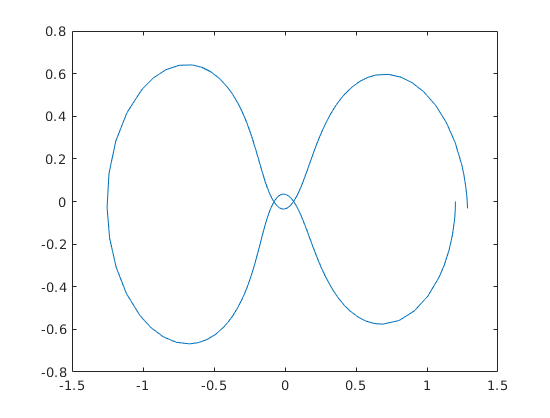
hold on
plot(u0(1),u0(3),'*b')    % Initial point. (b=blue)
% plot(x(1),y(1),'*b')    % Same as the previous line.
plot(x(end),y(end),'ko')  % Final point (k=black)
plot(-mu,0,'*k',lam,0,'or') % plot earth and moon  (r=red)
%legend('Orbit','Initial pt.','Final pt.','Earth','Moon')
grid on
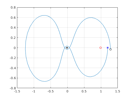
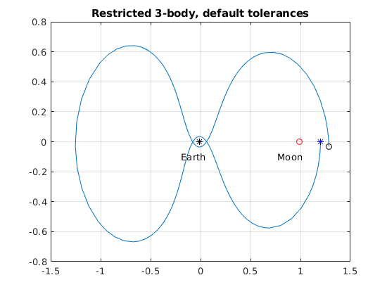
Text to plots (start with gtext, then change to text)
%gtext('Earth')        % Get text coordinates with mouse.
 text(-.2,-.1,'Earth')
% gtext('Moon')
 text(.77,-.1,'Moon')
 title('Restricted 3-body, default tolerances')
Adjust tolerances:
options=odeset('AbsTol',1e-6,'RelTol',1e-8);
options.Stats='on';
options
[T1,U1]=ode45(@Apollosys,Tspan,u0,options);
options =

  struct with fields:

              AbsTol: 1.0000e-06
                 BDF: []
              Events: []
         InitialStep: []
            Jacobian: []
           JConstant: []
            JPattern: []
                Mass: []
        MassSingular: []
            MaxOrder: []
             MaxStep: []
         NonNegative: []
         NormControl: []
           OutputFcn: []
           OutputSel: []
              Refine: []
              RelTol: 1.0000e-08
               Stats: 'on'
          Vectorized: []
    MStateDependence: []
           MvPattern: []
        InitialSlope: []

163 successful steps
15 failed attempts
1069 function evaluations
New options - New figure
figure;
clf
hold on
plot(U1(:,1),U1(:,3));shg  % Orbit: x=U1(:,1); y=U1(:,3);
plot(u0(1),u0(3),'*b')    % Initial point.
% plot(U1(1,1),U1(1,3),'*')  % Same as the previous line.
plot(U1(end,1),U1(end,3),'ko') % Final point
% Now is periodic at the accuracy of pic.
plot(-mu,0,'*k',lam,0,'or') % plot earth and moon
title('Restricted 3-body, new tolerances')
%legend('Orbit','Initial pt.','Final pt.','Earth','Moon')
grid on
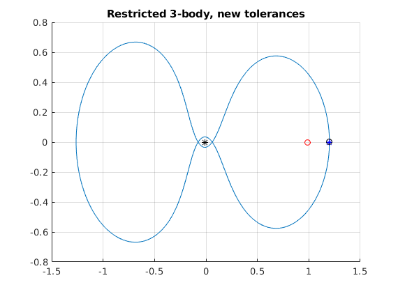
Smaller tolerances ==> Periodicity is shown at the accuracy of graphics.
Compute "periodicity error"
x1=U1(:,1);y1=U1(:,3);
deltax=x1(1)-x1(end);
deltay=y1(1)-y1(end);
dist=sqrt(deltax^2+deltay^2)    % Distance from initial point to final pt.
relerr=dist/x1(1)                %  Relative error
%       6.3511e-06      % So Periodic with about 6 numbers of accuracy.
%
dist =

   7.6214e-06


relerr =

   6.3511e-06
Next animate: (Skip now)
The simplest way for animation. For publish, comment this away
 %{
figure
axis([-1.5 1.5 -.8 .8]);
hold on
grid on
for j=1:length(T1)
    plot(x1(j),y1(j),'.r','MarkerSize',4)
    pause(0.01)   % adjust
end
 %}
% Don't need for-loop for "still" picture, just:
% plot(x1,y1,'or','MarkerSize',4) % The "still" picture command ...
%                                 % to be "decommented" for publish
%
For fun: animate the rays from earth to orbit.
(Remove comments if you like)
%{
for j=1:length(T1)
    plot([0 x1(j)],[0 y1(j)],'k')
    pause(0.005)   % adjust
end
%}
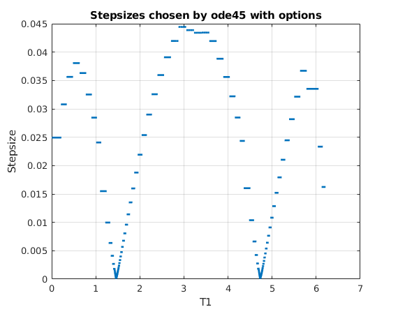
Look at stepsizes
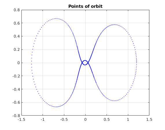
figure
%
% diff(T1) gives the difference vector:
% (T1(2)-T1(1),T1(3)-T1(2),...,T1(end)-T1(end-1)) % length=length(T1)-1
plot(T1(2:end),diff(T1),'.');grid on;shg
xlabel('T1')
ylabel('Stepsize')
title('Stepsizes chosen by ode45 with options')
figure
plot(x1,y1,'.b','MarkerSize',4)
title('Points of orbit')
grid on
% Zoom in to see that step sizes stay the same for a few steps usually.
% From the figure we see that the min and max stepsizes occur about at:
% t=1.5 and t=4.8 (min) and  t=0.5, 3, 5.7 (max)
%
More precise computaion with logical indexing etc. (skip here)
Do along ideas outlined in the commented block.
%{
[min1,ind1]=min(steps)
t1=T((T>1)&(T<3))
steps1=steps((T>1)&(T<3));
[min2,ind2]=min(steps1)
t2=t1(ind2)
hold on
plot(U1(ind2,1),U1(ind2,3),'*r')
%}
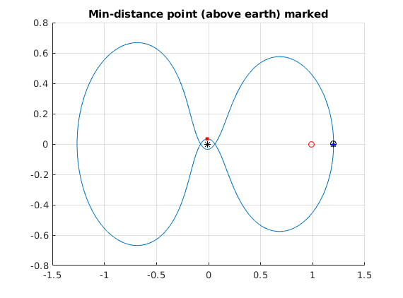
How close does the Apollo come to the surface of the earth?
Real sizes in kilometers:
distMoonEarth = 384400;
R_earth= 6371;
R_moon = 1737;
Distance to centre:
Find the minimum of
x=U1(:,1);
y=U1(:,3);
D2=y.^2+(x+mu).^2;
[minval2,minind]=min(D2);  % Finds the first minimum and its index.
xmin=x(minind);
ymin=y(minind);
minpoint=[xmin ymin]
minD=sqrt(minval2);
minDreal=minD*distMoonEarth
dist_to_surface_earth=minDreal-R_earth
%
minpoint =

   -0.0140    0.0346


minDreal =

   1.3317e+04


dist_to_surface_earth =

   6.9458e+03
Mark min distance point to figure(2)
figure(2)
hold on
plot(xmin,ymin,'.r','MarkerSize',10)
title('Min-distance point (above earth) marked')
Use logical indexing
Skip this part now.
%{
D2=@(x,y)y.^2+(x+mu).^2; % Define D2 as a function handle.
minval2=min(D2(x,y))
ind=D2(x,y)==minval2;
sum(ind)
%}
More fun:
ApollosolutionInteractive.m Interactive choice of initial points (like in dirfields earlier in the course)
Mathworks demo: orbitode contains advanced Matlab techniques, s.k. events. That gives a way to control the Timespan for various trajectories.